Creating a tomographic projection

Note

To keep the size of the documentation in version control manageable, we do not include images of the volume and the reconstruction. It is recommended to follow along in your favorite Python environment so you can see what is going on.

In this walkthrough, we will create tomographic projections using tomosipo. First, we import the necessary packages. By convention, tomosipo is imported as ts:

import tomosipo as ts
import numpy as np

Now we can create a volume and a circular parallel-beam projection geometry. The volume is a three-dimensional unit cube and is composed of 32 voxels in each dimension. The parallel-beam geometry has 32 angles that are equi-spaced over a half arc. The detector has 48 pixels in each dimension and has both height and width of 1.5 units.

vg = ts.volume(shape=(32, 32, 32), size=(1, 1, 1))
pg = ts.parallel(angles=32, shape=(48, 48), size=(1.5, 1.5))

If the size argument is omitted, a volume geometry uses unit voxel sizes, so its physical size matches its shape. See tomosipo.volume() for details. Similarly, projection geometries use unit detector pixels by default. Instead of specifying the number of angles, you can also pass an array of angles directly. See tomosipo.parallel() for more information.

The geometries have readable string representations, so we can inspect what we created:

>>> print(vg)
ts.volume(
    shape=(32, 32, 32),
    pos=(0.0, 0.0, 0.0),
    size=(1.0, 1.0, 1.0),
)
>>> pg    # or just press enter in the Python console..
ts.parallel(
    angles=32,
    shape=(48, 48),
    size=(1.5, 1.5),
)

In addition, we can display the geometry as an SVG animation:

svg = ts.svg(vg, pg)
svg.save("./doc/img/intro_forward_projection_geometries.svg")

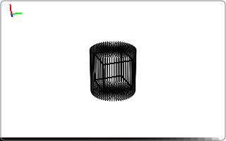
As you can see, in our geometry definition the detector overlaps with the volume. Although this is physically impossible, this is not a problem because the projection operator takes into account ray-volume intersections both behind and in front of the detector.

A projection operator can be created as follows:

A = ts.operator(vg, pg)

The operator has two useful properties, domain_shape and range_shape, which can be used to create volume and projection data:

>>> A.domain_shape, A.range_shape
((32, 32, 32), (48, 32, 48))
>>> x = np.ones(A.domain_shape, dtype=np.float32)

As you can see, the projection data is stored as a stack of sinograms, following the ASTRA-toolbox convention. The first dimension is the detector height, the second is the projection angle, and the third is the detector width.

Now, we can create a projection by applying the operator to the data x:

>>> y = A(x)
>>> y.shape
(48, 32, 48)

You can take a look at the projections using matplotlib.

import matplotlib.pyplot as plt
plt.imshow(y[:, 0, :]) # first projection
plt.imshow(y[:, 8, :]) # quarter rotation

Proceed to the next tutorial to see how to compute a reconstruction from these projection data.