Hyperparameter Tuning
Introduction
Hyperparameter tuning is a crucial step in the process of regularized reconstruction. The goal is to find the optimal hyperparameters that balance the trade-off between data fidelity and regularization. The data fidelity term measures the discrepancy between the reconstructed image and the measured data, while the regularization term enforces a desired property on the reconstructed image, such as smoothness or sparsity. In the context of regularized reconstruction, the hyperparameter of interest is typically the regularization weight (λ). The regularization weight controls the strength of the regularization term in the objective function, thus controlling the trade-off between these two terms. A too high regularization weight results in a over-regularized reconstruction, while a too low regularization weight results in a noisier (under-regularized) reconstruction. The objective function can be expressed as the following: \( \min_x \frac{1}{2} \lVert Ax - b \rVert_2^2 + \lambda R(x)\), where \(R: \mathbb{R}^N \rightarrow \mathbb{R}\) denotes a regularization term, \(A: \mathbb{R}^N \rightarrow \mathbb{R}^M\) is the forward operator, \(\hat{x} \in \mathbb{R}^{N}\) the sought reconstruction, and \(b \in \mathbb{R}^{M}\) the measured data (with \(N\) the number of unknowns and \(M\) the number of measurements).
The module param_tuning provides a couple of methods to find the best regularization weight, according to the metrics defined by the user. To work with this module, we need to first define a reconstruction function that accepts the lambda value as input. Depending on the method, the function might also need to accept a data mask, which allows the method to mask certain data points (e.g., the cross-validation method). Here below is an example:
def solve_reg(lam_reg: float, b_test_mask: NDArray | None = None) -> tuple[NDArray, SolutionInfo]:
    solver = cct.solvers.PDHG(
        verbose=True, data_term=data_term_lsw, regularizer=reg(lam_reg), data_term_test=data_term_lsw, leave_progress=False
    )
    with cct.projectors.ProjectorUncorrected(ph.shape, angles) as prj:
        return solver(prj, sino_substr, iterations, x_mask=vol_mask, lower_limit=lower_limit, b_test_mask=b_test_mask)
This function will then be passed to the method of choice to compute the corresponding merit function values. In fact, each method will have a different way of testing the quality of each reconstruction and then select the best one.
We also need to define the lambda values to test, and this can be done with the utility function get_lambda_range, like the following:
lams_reg = cct.param_tuning.get_lambda_range(1e-3, 1e1, num_per_order=4)
L-curve Method
The L-curve method is a popular approach for hyperparameter tuning in regularized reconstruction. The L-curve method involves plotting the regularization parameter (λ) against corresponding objective function values, computed over a merit function of interest. This means that each reconstruction is evaluated with a specific function which associates a cost to it. Here, we will use the total variation (TV) semi-norm.
The L-curve method is based on the observation that the optimal regularization parameter corresponds to the “corner” of the L-curve. The corner of the L-curve represents the point where the objective function value starts to increase rapidly. This point corresponds to the optimal balance between data fidelity and regularization.
In the provided code, the L-curve method is implemented in the LCurve class. The LCurve class takes a loss function as input, which is used to compute the objective function values for different regularization parameters. The compute_loss_values method of the LCurve class computes the objective function values for a range of regularization parameters. The plot_result method of the LCurve class plots the L-curve, which can be used to identify the optimal regularization parameter.
# Set up the required functions
def iso_tv_seminorm(x: NDArray) -> float:
    """Compute the isotropic TV semi-norm.

    Used in the L-curve.

    Parameters
    ----------
    x : NDArray
        Input array.

    Returns
    -------
    float
        The isotropic TV semi-norm of the input array.
    """
    op = cct.operators.TransformGradient(x.shape)
    d = op(x)
    d = np.linalg.norm(d, axis=0, ord=2)
    return float(np.linalg.norm(d.flatten(), ord=1))

# Create the regularization weight finding helper object (using L-curve)
hpt_lc = cct.param_tuning.LCurve(iso_tv_seminorm, verbose=True, plot_result=True)
hpt_lc.task_exec_function = solve_reg

f_vals_lc = hpt_lc.compute_loss_values(lams_reg)
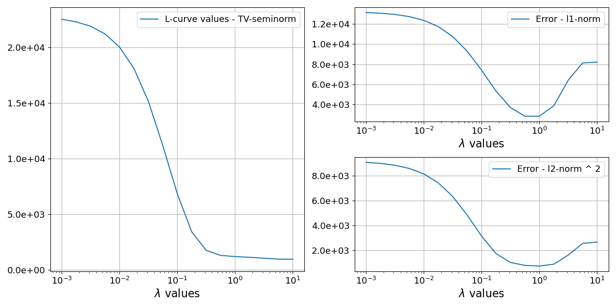
Here above, we show an example of L-curve loss plot, where the convex “corner” of the curve is the usual point where one would want to select the lambda value.
Cross-Validation Method
The cross-validation (CV) method is another popular approach for hyperparameter tuning in regularized reconstruction. The CV method involves splitting the data into training and validation sets. The training set is used to compute the regularized reconstruction, while the validation set is used to evaluate the quality of the reconstruction. The CV method is based on the observation that the optimal regularization parameter corresponds to the point where the reconstruction error on the validation set is minimized. The reconstruction error is typically computed using a metric such as the mean squared error (MSE) or the mean absolute error (MAE).
Definitions of the Sets
Let the full measurement set be represented by the forward operator \(A\) and the measured data \(b\). These are partitioned as follows:
Reconstruction set: \(A_{\text{r}}\), \(b_{\text{r}}\)
Cross-validation set: \(A_{\text{cv}}\), \(b_{\text{cv}}\)
These sets are complementary, meaning: \( A = \begin{bmatrix} A_{\text{r}} \\ A_{\text{cv}} \end{bmatrix}, \quad b = \begin{bmatrix} b_{\text{r}} \\ b_{\text{cv}} \end{bmatrix} \)
Regularized Reconstruction Problem
The regularized reconstruction is computed using the reconstruction set, with the objective function:
\(
\min_{x} \left\{ \frac{1}{2} \|A_{\text{r}}x - b_{\text{r}}\|_2^2 + \lambda R(x) \right\}
\)
where:
\(A_{\text{r}}\) is the forward operator for the reconstruction set,
\(b_{\text{r}}\) is the measured data for the reconstruction set,
\(x\) is the reconstructed image,
\(R(x)\) is the regularization term (e.g., \(\| \, |\nabla x | \, \|_1\) for the TV semi-norm),
\(\lambda\) is the regularization weight.
Cross-Validation Objective Function
The cross-validation objective function evaluates the quality of the reconstruction \(x(\lambda)\) (obtained for a given \(\lambda\)) on the cross-validation set:
\(
f(\lambda) = \frac{1}{2} \|A_{\text{cv}}x(\lambda) - b_{\text{cv}}\|_2^2
\)
where:
\(A_{\text{cv}}\) is the forward operator for the cross-validation set,
\(b_{\text{cv}}\) is the measured data for the cross-validation set,
\(x(\lambda)\) is the reconstructed image for a given \(\lambda\).
The goal of the CV method is to find the regularization weight \(\lambda\) that minimizes the cross-validation objective function \(f(\lambda)\). This ensures that the chosen \(\lambda\) generalizes well to unseen data, as the cross-validation set is not used during the reconstruction process.
The CV method is implemented in the CrossValidation class. This class takes the data shape and the number of averages as input. Its compute_loss_values method computes the cross-validation loss values for a range of regularization parameters. The fit_loss_min method is used to estimate the best regularization parameter, by fitting a parabola around the lowest loss curve value and identifying the vertex position of the parabola (i.e., its minimum) as the optimal regularization parameter.
# Create the regularization weight finding helper object (using cross-validation)
hpt_cv = cct.param_tuning.CrossValidation(sinogram.shape, verbose=True, num_averages=3)
hpt_cv.task_exec_function = solve_reg

# Define the regularization weight range
lams_reg = cct.param_tuning.get_lambda_range(1e-3, 1e1, num_per_order=4)

# Compute the loss function values for all the regularization weights
f_avgs, f_stds, _ = hpt_cv.compute_loss_values(lams_reg)

# Compute the error values for all the regularization weights
err_l1, err_l2 = hpt_cv.compute_reconstruction_error(lams_reg, expected_ph)

# Parabolic fit of minimum over the computer curve
lam_min, _ = hpt_cv.fit_loss_min(lams_reg, f_avgs)
As mentioned above, the task execution function should accept an extra parameter, which takes the data mask indicating the cross-validation values. This parameter is conventionally called b_test_mask for historical reasons. It’s name can be changed, provided that it is also passed to the argument mask_param_name of the CrossValidation class.
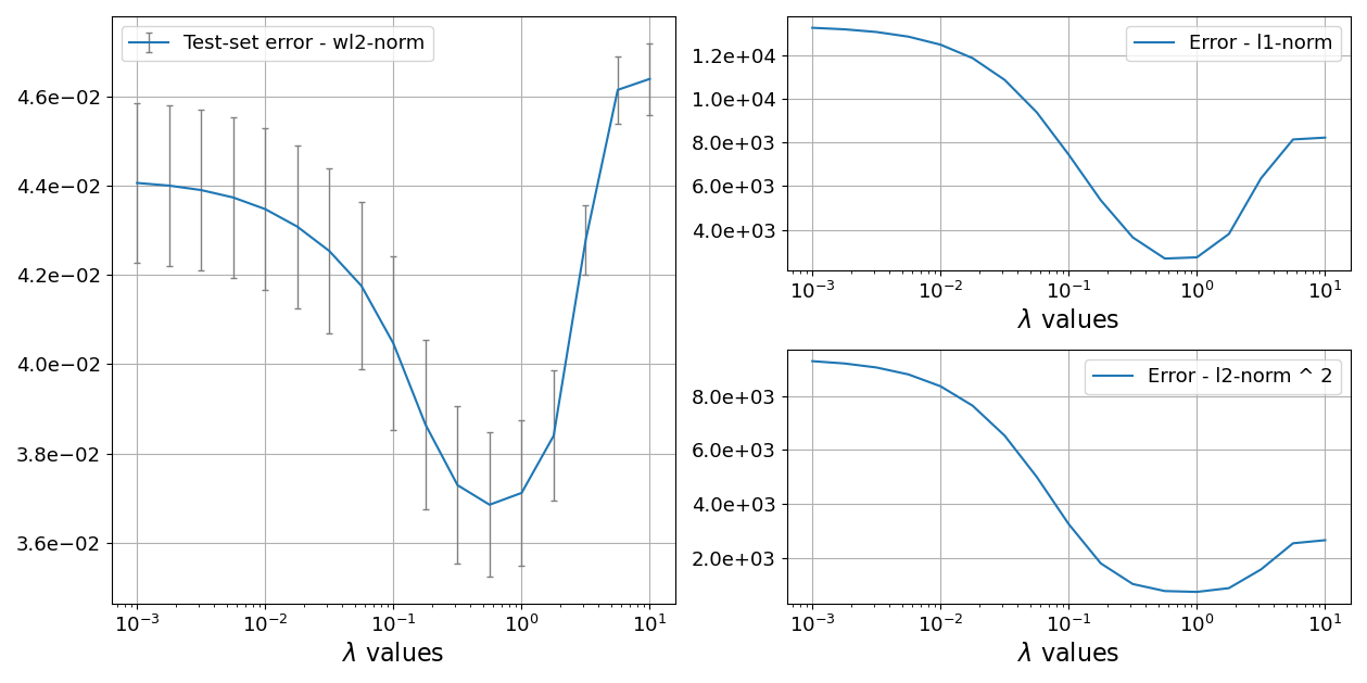
Here above, we show an example of the cross-validation loss plot, which is presented alongside the reconstruction error of the corresponding reconstructions (both computed with the \(l_2\) and \(l_1\) norms). The highest fidelity reconstruction (according to the minimum of the reconstruction error) is in the neighborhood of the lowest cross-validation loss value.
k-Fold Cross-Validation
A popular extension of the CV method is k-fold cross-validation, where the full dataset is divided into \(k\) equally sized folds. The reconstruction and validation process is repeated \(k\) times, each time using a different fold as the cross-validation set and the remaining \(k-1\) folds as the reconstruction set. The final regularization parameter \(\lambda\) is selected based on the average performance across all \(k\) folds. This approach reduces variance in the estimate of the optimal \(\lambda\) and provides a more robust evaluation of the model’s generalization ability.
k-Fold CV can be achieved by setting the cv_fraction parameter to None in the initialization of the CrossValidation class, which will then use the function create_k_fold_test_masks to create the data masks. The number of folds will be determined by the parameter num_averages, which is equal to 5 by default. For more details we refer to scikit-Learn’s excellent explanation.
Parallelization & distributed computation
It is possible to accelerate the computation of the objective function values by using parallelization. This can be achieved by setting the parallel_eval parameter to one of the following values: True, an int, or an Executor object. If parallel_eval is set to True, the number of parallel threads will be determined by the number of available CPUs. If parallel_eval is set to an integer, the number of parallel threads will be set to that value. If parallel_eval is set to an Executor object, the Executor object will be used to parallelize the computation. Examples of Executor objects are ThreadPoolExecutor, ProcessPoolExecutor, or the Executor-like object returned by distributed’s Client.get_executor() method. For more details on parallelization, we refer to the concurrent.futures module and the distributed library.
Here is an example of how to use a distributed cluster to parallelize the computation of the objective function values:
from distributed import LocalCluster, Client

with LocalCluster(n_workers=4, threads_per_worker=1) as cluster, Client(cluster) as client:
    hpt_cv = cct.param_tuning.CrossValidation(
        sinogram.shape, verbose=True, num_averages=3, parallel_eval=client.get_executor()
    )
    hpt_cv.task_exec_function = solve_reg

    # Compute the loss function values for all the regularization weights
    f_avgs, f_stds, _ = hpt_cv.compute_loss_values(lams_reg)
Beware that every NDArray (even hidden inside another object) that is passed to the solve_reg closure should be copied to avoid race conditions.
Thus, the function should be modified as follows:
from copy import deepcopy

def solve_reg(lam_reg: float, b_test_mask: NDArray | None = None) -> tuple[NDArray, SolutionInfo]:
    solver = cct.solvers.PDHG(
        verbose=True,
        data_term=deepcopy(data_term_lsw),
        regularizer=reg(lam_reg),
        data_term_test=deepcopy(data_term_lsw),
        leave_progress=False,
    )
    with cct.projectors.ProjectorUncorrected(ph.shape, angles) as prj:
        return solver(
            prj,
            sino_substr.copy(),
            iterations,
            x_mask=vol_mask.copy(),
            lower_limit=lower_limit,
            b_test_mask=b_test_mask.copy()
        )
Dedicated task initialization function support
The LCurve and CrossValidation classes support passing a dedicated initialization function, alongside the execution function (task_init_function and task_exec_function respectively). This is useful when the initialization of the task could benefit from being implemented in a separate function, for example to avoid making the task execution function too complex, to acquire more granular execution timings, or to just keep the two business logics separate.
The initialization function should be a callable that takes the lambda value as first argument, while now the task execution function should take the output of the initialization function as first argument. Here below is an example:
# Instantiates the solver object, that is later used for computing the reconstruction
def solver_init(lam_reg: float):
    # Using the PDHG solver from Chambolle and Pock
    return cct.solvers.PDHG(
        verbose=True, data_term=data_term_lsw, regularizer=reg(lam_reg), data_term_test=data_term_lsw, leave_progress=False
    )

# Computes the reconstruction for a given solver and a given cross-validation data mask
def solver_exec(solver, b_test_mask: NDArray | None = None):
    with cct.projectors.ProjectorUncorrected(ph.shape, angles) as prj:
        return solver(prj, sino_substr, iterations, x_mask=vol_mask, lower_limit=lower_limit, b_test_mask=b_test_mask)

print("Reconstructing:")
# Create the regularization weight finding helper object (using cross-validation)
hpt_cv = cct.param_tuning.CrossValidation(sinogram.shape, verbose=True, num_averages=3)
hpt_cv.task_init_function = solver_init
hpt_cv.task_exec_function = solver_exec
Computation performance metrics
It is possible to obtain computation performance metrics, by setting the parameter print_timings to True. At the end of each computation batch, the LCurve and CrossValidation classes will print the total batch time, broken into initialization, and total execution, alongside the average task time. When using the two-function approach, the execution time will also correctly report the time spent in the initialization function and the execution function, respectively.
The output will look like this:
Performance Statistics:
- Initialization time: 00:00:00.007
- Processing time: 00:00:13.949
- Total time: 00:00:13.956 (Tasks/Total ratio: 6.27)

Average Task Performance:
- Initialization time: 00:00:00.000
- Execution time: 00:00:05.142
- Total time: 00:00:05.142
The Tasks/Total ratio indicates the ratio between the total execution time and the total time spent in the task functions. This ratio is useful to estimate the speed-up that was obtained by parallelizing the task execution. It does not take reduced performance due to resource contention between the tasks, so it should be taken only as an approximate indication of the parallelization efficiency.
It is also possible to return this information in the form of PerfMeterBatch and list[PerfMeterBatch] when passing the argument return_all=True to the compute_loss_values method. This allows for more detailed analysis of the performance of the parallel execution by the user.
Complete code example
For a complete code example on how to use the LCurve and CrossValidation classes to perform hyperparameter tuning for regularized reconstruction, we refer to the script: examples/example_06_guided_regularization.py. The code first sets up the required functions and initializes the objects and the search range for the hyperparameter. It then computes the objective function values and the reconstruction error for a range of regularization parameters. Finally, it visualizes the results.