Attenuation correction

In this tutorial, we show how to use corrct’s attenuation correction functions. We first create a synthetic test case, as the one presented in:

• N. Viganò and V. A. Solé, “Physically corrected forward operators for induced emission tomography: a simulation study,” Meas. Sci. Technol., no. Advanced X-Ray Tomography, pp. 1-26, Nov. 2017.

Synthetic data creation

We can create the phantom and the local attenuation coefficient maps for the incoming beam and emitted photon energies with the following code:

try:
    import phantom
except ImportError:
    cct.testing.download_phantom()
    import phantom

vol_shape = [256, 256, 3]

ph_or = np.squeeze(phantom.modified_shepp_logan(vol_shape).astype(np.float32))
ph_or = ph_or[:, :, 1]

ph, vol_att_in, vol_att_out = cct.testing.phantom_assign_concentration(ph_or)

These are the resulting images:

Image

Code

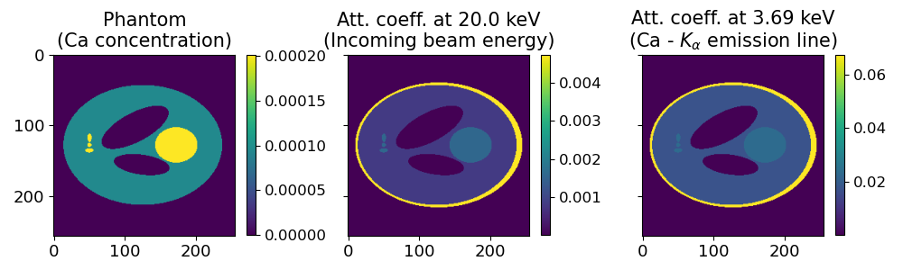
out_energy = cct.physics.xrf.get_energy("Ca", "KA", compute_average=True)

fig, axs = plt.subplots(1, 3, sharex=True, sharey=True, figsize=(10, 3))
im = axs[0].imshow(ph)
axs[0].set_title("Phantom\n(Ca concentration)", fontsize=15)
cbar = plt.colorbar(im, shrink=0.83)
cbar.ax.tick_params(labelsize=12)
im = axs[1].imshow(vol_att_in)
axs[1].set_title(f"Att. coeff. at {20.0:.3} keV\n(Incoming beam energy)", fontsize=15)
cbar = plt.colorbar(im, shrink=0.83)
cbar.ax.tick_params(labelsize=12)
im = axs[2].imshow(vol_att_out)
axs[2].set_title(f"Att. coeff. at {out_energy:.3} keV\n(Ca - $K_\\alpha$ emission line)", fontsize=15)
cbar = plt.colorbar(im, shrink=0.83)
cbar.ax.tick_params(labelsize=12)
for ax in axs:
    ax.tick_params(labelsize=13)
fig.tight_layout()

Where the first on the left, is the local mean XRF photon production of the \(K_{\alpha}\) emission line of Ca, the second is the local linear attenuation for the incoming beam (at 20 keV), and the last one is the local linear attenuation for the emitted photons (at 3.69 keV). It should be noted that the local linear attenuations used here are the result of \(\mu \cdot d\), where \(d\) is the voxel size, and \(\mu\) the local linear attenuation coefficient at the respective given energies.

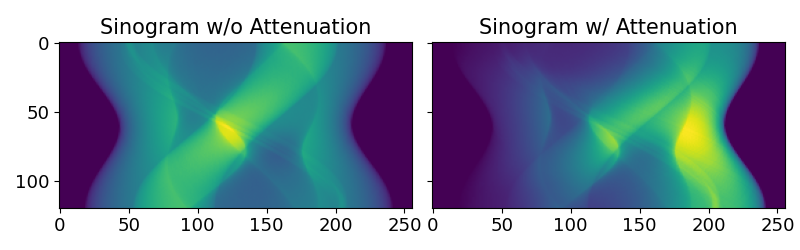
We then create a sinogram with the following function:

sino, angles_rad, expected_ph, _ = cct.testing.create_sino(ph, 120, vol_att_in=vol_att_in, vol_att_out=vol_att_out, psf=None)

Since the XRF detector is supposed to be on the right side of the sinogram, it will show strong attenuation effects on the side that is the most far away (left). Here below is a comparison against a non-attenuated sinogram.

Image

Code

fig, axs = plt.subplots(1, 2, sharex=True, sharey=True, figsize=(8, 2.5))
axs[0].imshow(sino_noatt)
axs[0].set_title("Sinogram w/o Attenuation", fontsize=15)
axs[1].imshow(sino)
axs[1].set_title("Sinogram w/ Attenuation", fontsize=15)
for ax in axs:
    ax.tick_params(labelsize=13)
fig.tight_layout()

Computing local attenuation maps

Given the known sample composition, the local attenuation maps can be computed with the following code, which is also used in the function testing.phantom_assign_concentration:

volume_obj = physics.VolumeMaterial(materials_fractions, materials_compound_names, voxel_size_cm)

vol_lin_att_in = volume_obj.get_attenuation(in_energy_keV)
vol_lin_att_out = volume_obj.get_attenuation(out_energy_keV)

where materials_fractions is a list of volumes containing the local concentration fraction of each material present in the sample volume, and materials_compound_names is a list of compound names for each corresponding material. The function get_attenuation of the volume_obj object is then used to compute the local linear attenuation for the incoming and outgoing X-ray energies, as returned by the function testing.phantom_assign_concentration.

Reconstruction

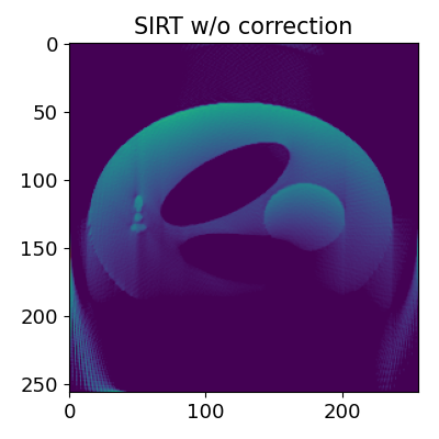
When proceeding to reconstruct with an uncorrected project as the following:

solver_sirt = cct.solvers.SIRT(verbose=True)

vol_geom = cct.models.get_vol_geom_from_data(sino)

with cct.projectors.ProjectorUncorrected(vol_geom, angles_rad) as p:
    rec_sirt_uncorr, _ = solver_sirt(p, sino, iterations=250, lower_limit=0.0)

We obtain the following reconstruction:

If instead we use a corrected projector with the following code:

with cct.projectors.ProjectorAttenuationXRF(vol_geom, angles_rad, att_in=vol_att_in, att_out=vol_att_out) as p:
    rec_sirt_corr, _ = solver_sirt(p, sino, iterations=250, lower_limit=0.0)

We obtain a corrected reconstruction:

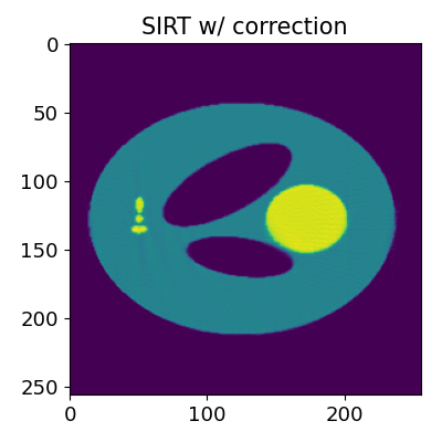
The resulting reconstruction still shows some imperfections, but most of the aberrations have been corrected.

What happens behind the scenes

What the project projectors.ProjectorAttenuationXRF actually does is to compute local attenuation maps for the pixels at each reconstruction angle. This can be seen if we directly use the physics.attenuation.AttenuationVolume class, instead of letting the projector call it for us:

att = cct.physics.attenuation.AttenuationVolume(
    incident_local=vol_att_in, emitted_local=vol_att_out, angles_rot_rad=angles_rad
)
att.compute_maps()

Two of the maps computed with the physics.attenuation.AttenuationVolume.compute_maps method are shown here below:

Image

Code

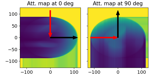
fig, axs = plt.subplots(1, 2, sharex=True, sharey=True, figsize=(6, 3))
att.plot_map(axs[0], rot_ind=0)
axs[0].set_title("Att. map at 0 deg", fontsize=15)
att.plot_map(axs[1], rot_ind=60)
axs[1].set_title("Att. map at 90 deg", fontsize=15)
for ax in axs:
    ax.tick_params(labelsize=13)
fig.tight_layout()

The red arrow indicates the incoming beam direction, while the black arrow indicates the XRF detector position with respect to the sample.

These maps can then be passed to the projector with the **att.get_projector_args() method:

with cct.projectors.ProjectorAttenuationXRF(ph.shape, angles_rad, **att.get_projector_args()) as p:
    rec_sirt_corr, _ = solver_sirt(p, sino, iterations=250, lower_limit=0.0)