Denoising images¶

Modelling¶

All models are wrong, but some are useful.

- George Box

What is an image¶

Mathematicians like to think of images as vector-valued functions
Computer scientists like to think of images as multi-dimensional arrays
We can even think of images as graphs

For today, we focus on grey-scale images represented as 2D arrays $F \in \mathbb{R}^{n\times n}$ or 1D arrays $\mathbf{f}\in\mathbb{R}^{n^2}$.

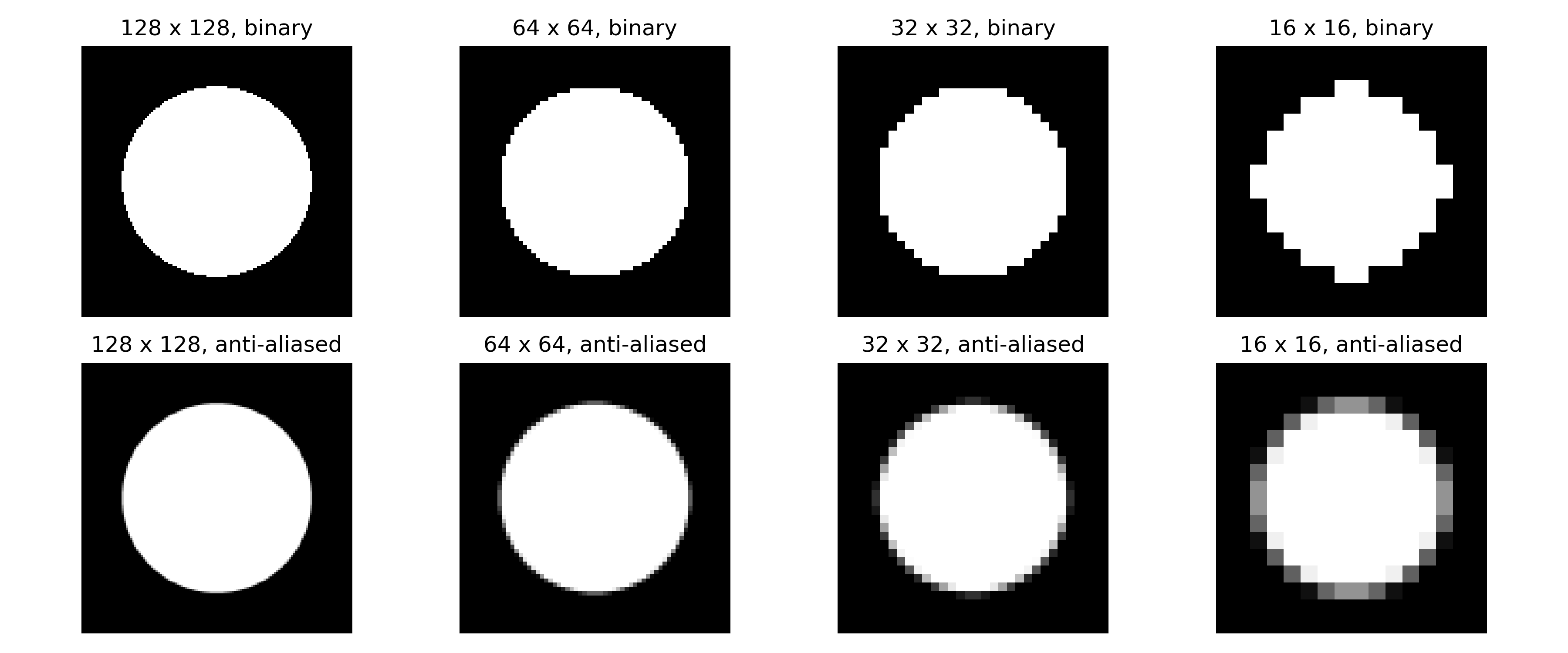
Images are typically represented as piece-wise constant on a grid of square pixels (this is often called rasterization)
Rasterization leads to issues when representing objects with sharp boundaries
Compare binary rasterization (the signal is sampled at the center of each pixel) with anti-aliased version (the signal is averaged over the area of each pixel)
In practice, rasterization is defined by the imaging system

Types of noise¶

We can think of noise as any feature in the image that diminishes its scientific usefulness
This could include measurement noise, distortions, pre-processing artifacts, quantization, ...
We will focus on noise that can be modelled stochastically, as perturbation of underlying "clean" image.

Additive Gaussian noise:

$$f_i\sim N (\overline{f}_i,\sigma^2)$$

Poisson noise:

$$f\sim P(\overline{f}_i)$$

Salt-and-Pepper:

$$f_i = \begin{cases} 0 & \text{with probability } p/2 \\ 1 & \text{with probability } p/2\\ \overline{f}_i & \text{with probability } 1-p \end{cases}$$

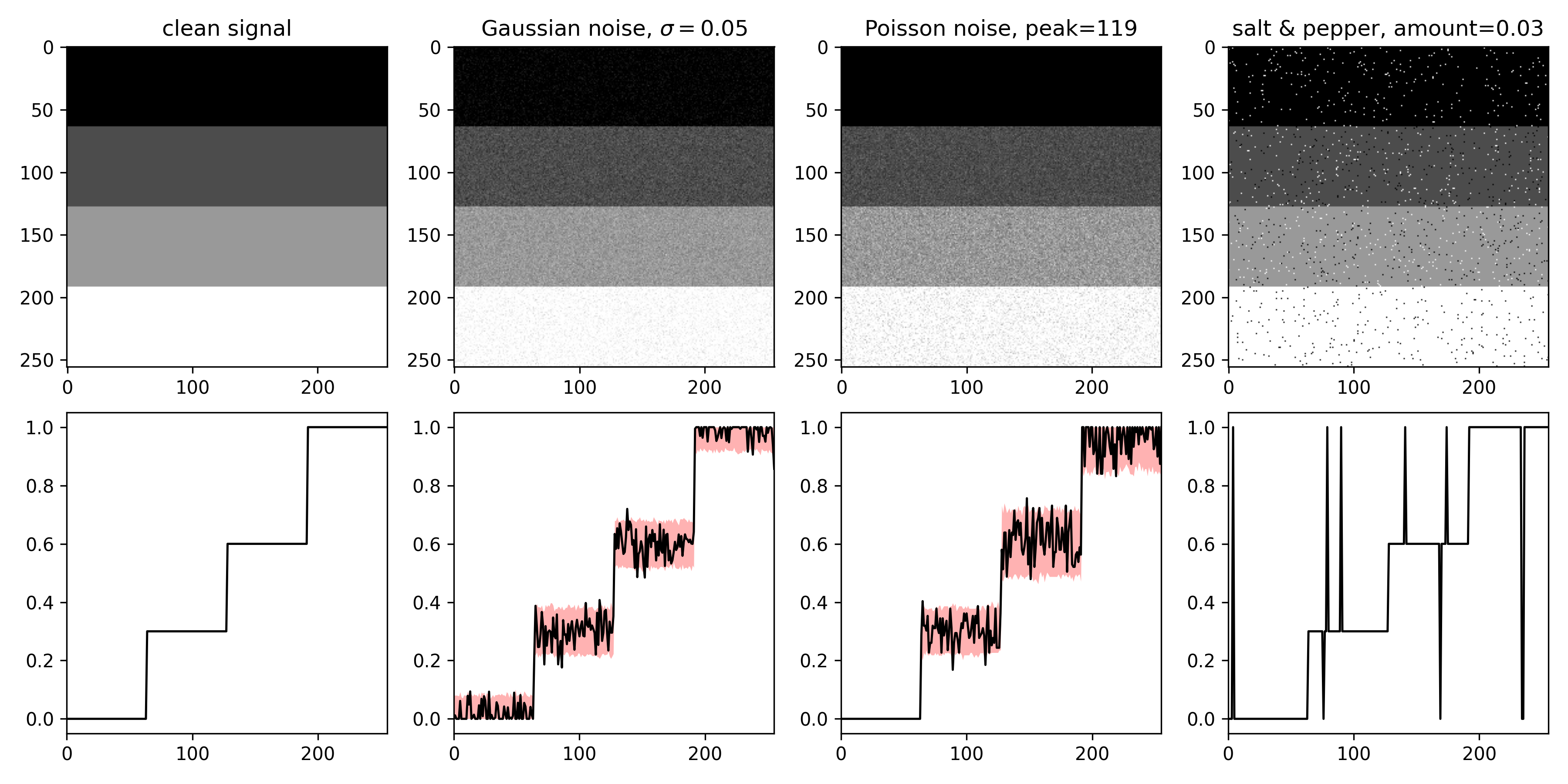
Note the truncation of the signal. It's an additional factor complicating the noise model!

How do we compare images?¶

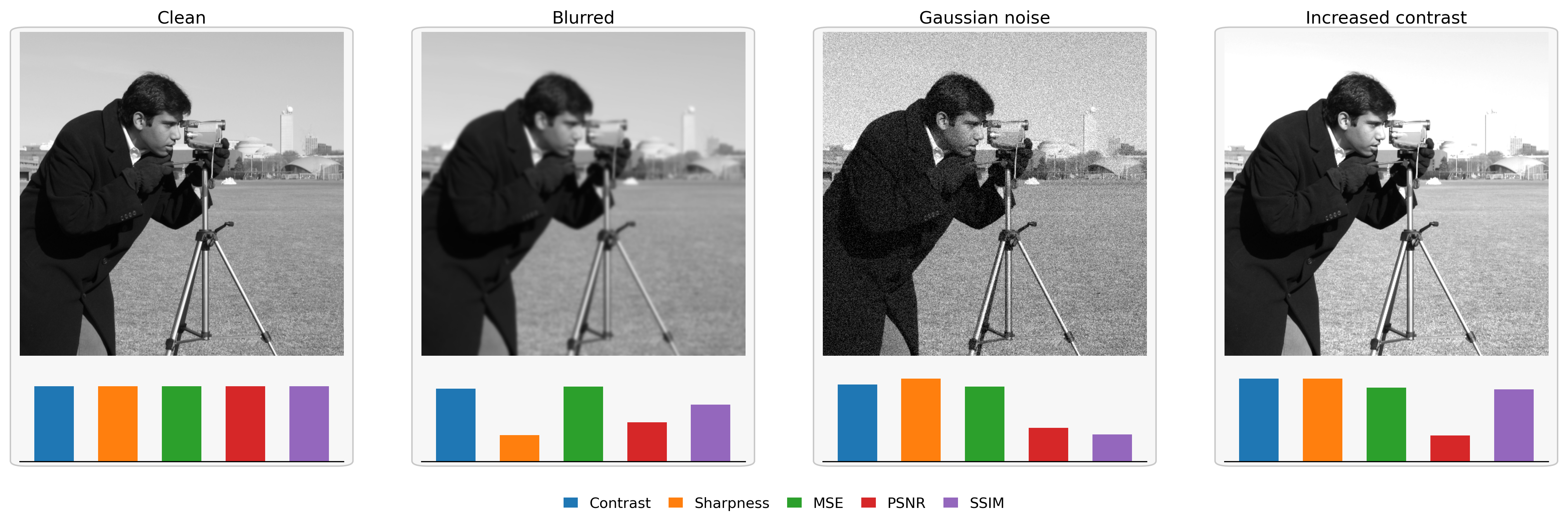
We need a way to judge the quality of an image. Which metric is suitable is highly application (and community) dependent.

We discern methods with and without a reference:

Without : resolution, contrast, ...
With : signal-to-noise ratio (SNR), mean squared error (MSE), structural similarity (SSIM), log-likelihood

Getting rid of noise¶

Getting rid of noise is easy, it's keeping the useful bits that is hard.

- This lecture

Bias and variance¶

Suppose we have a noisy version, $F^\delta$, of $\overline{F}$ and a method to denoise the image: $$\widetilde{F} = \mathcal{R}(F^\delta).$$

If $\mathcal{D}$ is a metric we can decompose the error as $$\mathbb{E} \mathcal{D}\bigl(\mathcal{R}(F^\delta),\overline{F}\bigr) \leq \underbrace{\mathcal{D}\bigl(\mathcal{R}(\overline{F}),\overline{F}\bigr)}_{\text{bias}} + \underbrace{\mathbb{E} \mathcal{D}\bigl(\mathcal{R}(F^\delta),\mathcal{R}(\overline{F})\bigr)}_{\text{variance}}.$$

Bias is what the method gets wrong even on a clean image, for example by smoothing away real detail.
Variance is how much the output changes when the noise realization changes: a very sensitive method has high variance.

The ideal denoiser has both a small bias and is stable.

These are conflicting goals
The stability of classical approaches is well-understood, but they may have a large bias
Learned approaches (next tutorial) may have a smaller bias but can be very unstable

Filtering and smoothing¶

Local (Gaussian) smoothing
Median filtering
Frequency-domain filtering

Local smoothing:

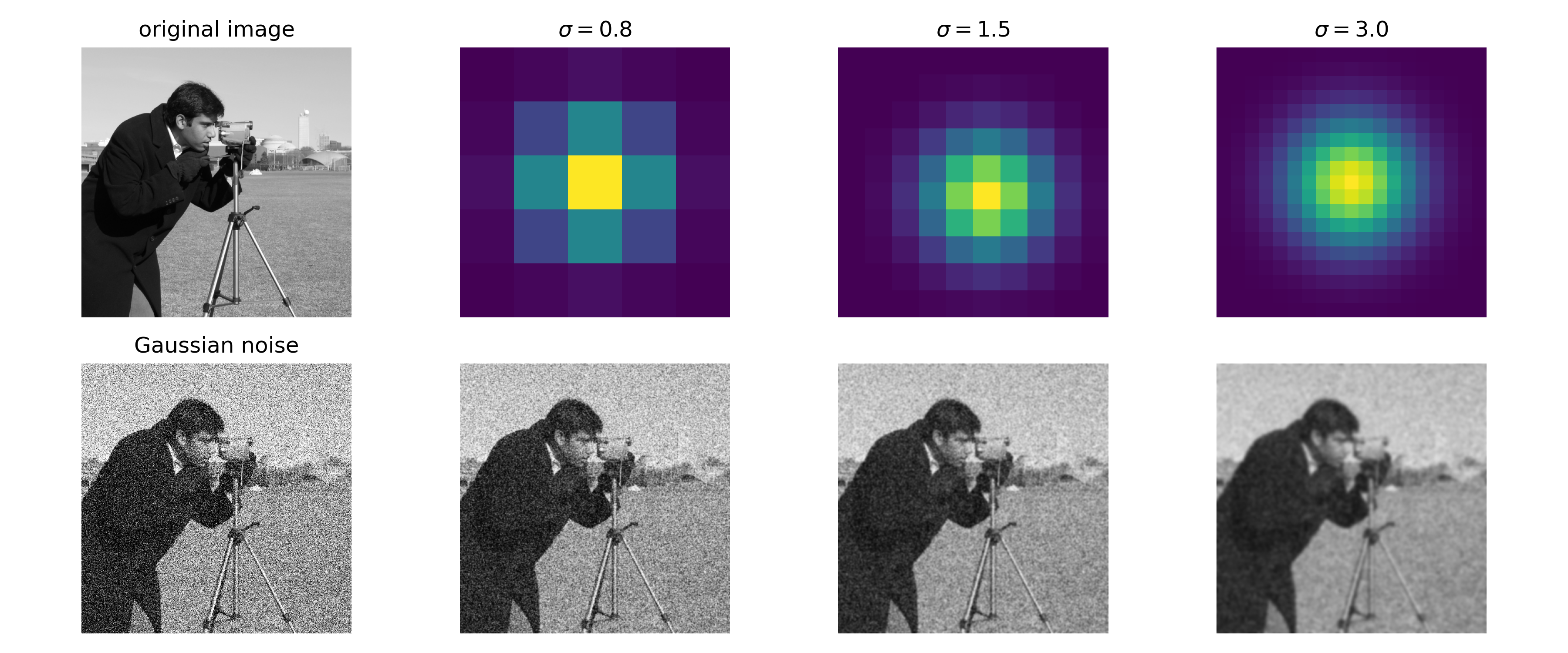
Noise fluctuates on a pixel-by-pixel basis, while the underlying image is highly correlated
This motivates local smoothing $$\widetilde{F}_{ij} = \sum_{k\ell} G_{|i-k|,|j-\ell|} F_{k\ell}^\delta$$

Gaussian filter

The Gaussian filter kernel: $G_{pq} = \frac{1}{2\pi\sigma^2} e^{-\frac{p^2 + q^2}{2\sigma^2}}$

Theoretical analysis

Based on assumptions that we make on the noise, we can analyse the accuracy of such a filter.

For example, let's use a simple five-point filter: $$\widetilde{F}_{i,j} =(1-4\alpha)F_{i,j}^\delta + \alpha(F_{i+1,j}^\delta + F_{i-1,j}^\delta + F_{i,j+1}^\delta + F_{i,j-1}^\delta)$$

Assuming that $F^\delta_{ij} \sim N(\overline{F}_{ij},\sigma^2)$ we have $$\mathbb{E}\|\widetilde{F} - \overline{F}\|_2^2 \leq \left(1 - 8\alpha + 20\alpha^2\right)n^2\sigma^2 + \alpha^2 \|\nabla^2 \overline{F}\|_2^2.$$
Assuming that $F^\delta_{ij} \sim \text{Poisson}(\overline{F}_{ij})$ we have $$\mathbb{E}\|\widetilde{F} - \overline{F}\|_2^2 \leq \left(1 - 8\alpha + 20\alpha^2\right)\|\overline{F}\|_1 + \alpha^2 \|\nabla^2 \overline{F}\|_2^2.$$

Simulated experiment

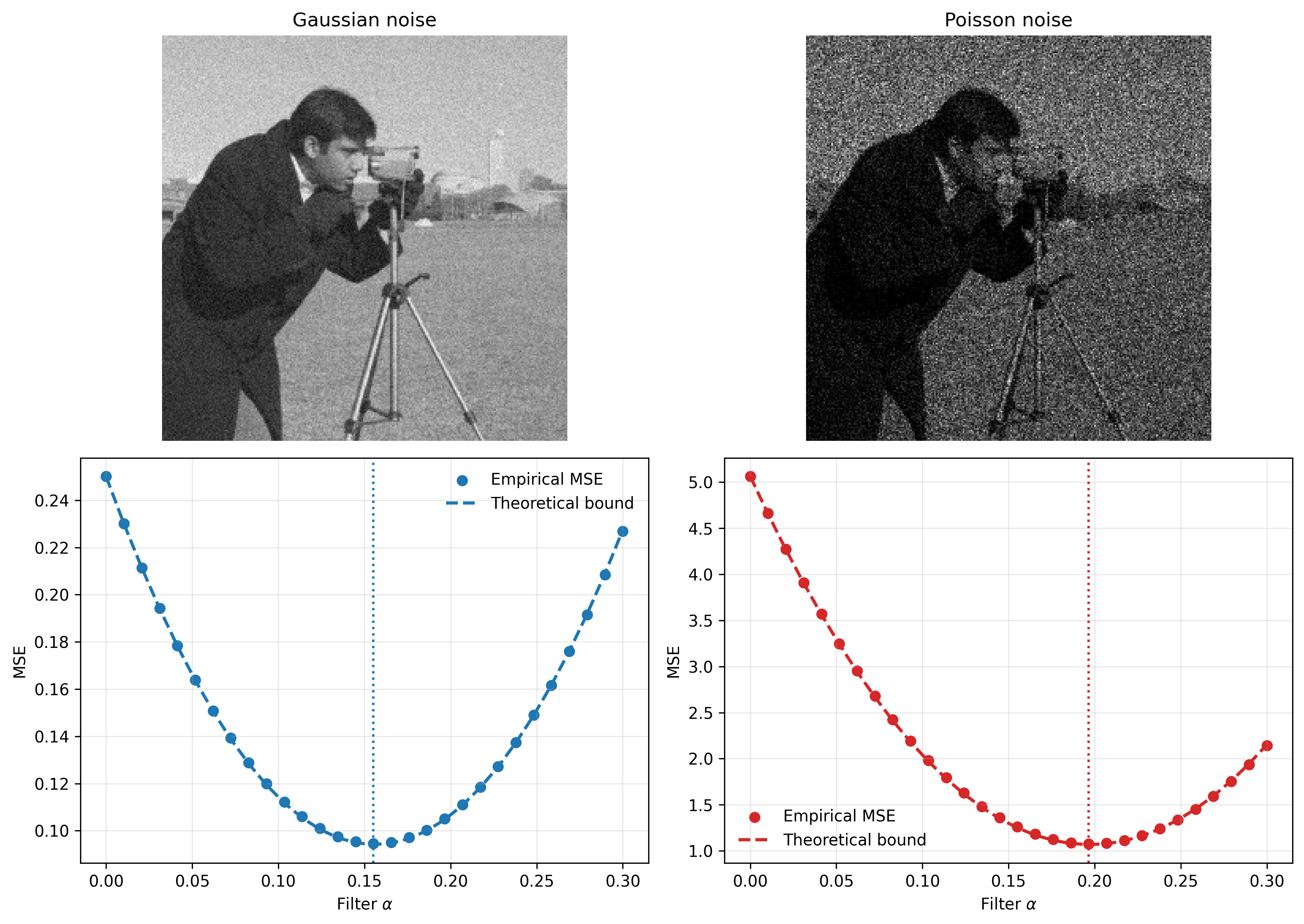
Trade-off between variance reduction and bias for the five-point filter

The dashed curves show the theoretical upper error bounds, while the points are empirical averages over repeated noise realisations.
Small $\alpha$ reduces variance, while larger $\alpha$ increases bias for the five-point filter.
With more noise, the optimal $\alpha$ is larger (more smoothing).

Median filter

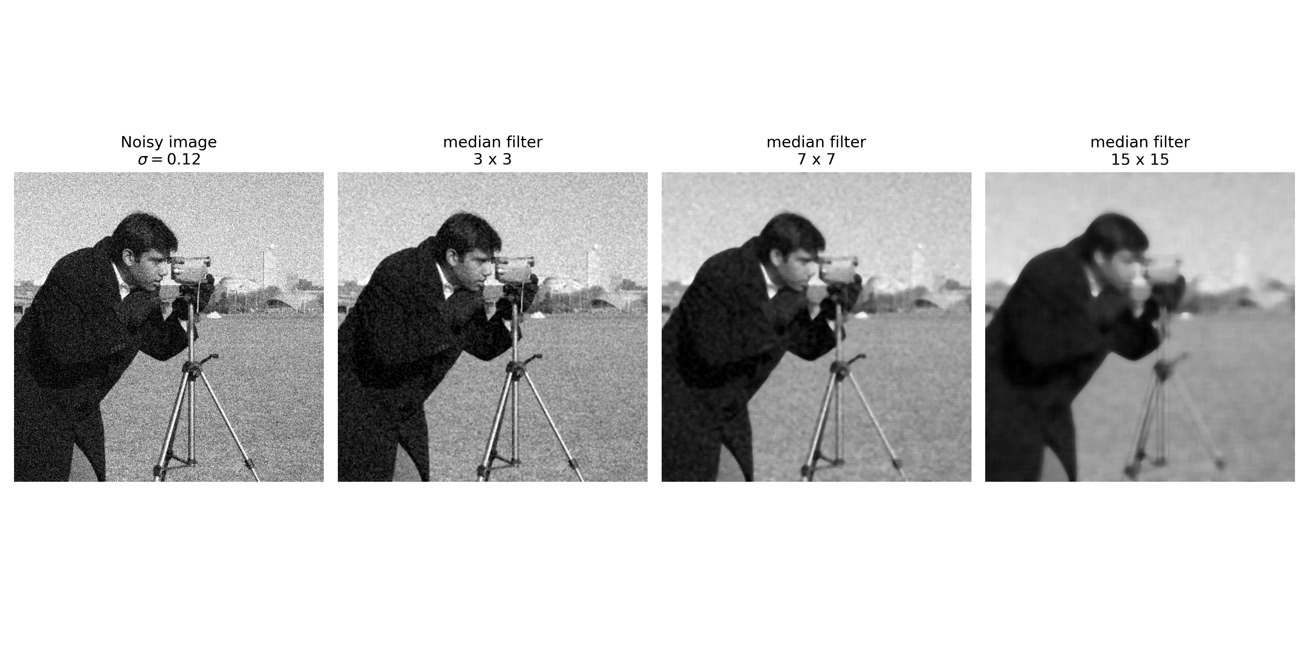
A disadvantage of the previous approach is that it also smoothes out edges in the image.
An alternative method is the median filter, which replaces the value in each pixel with the median of its neighborhood (instead of the weighted mean).

Fourier domain

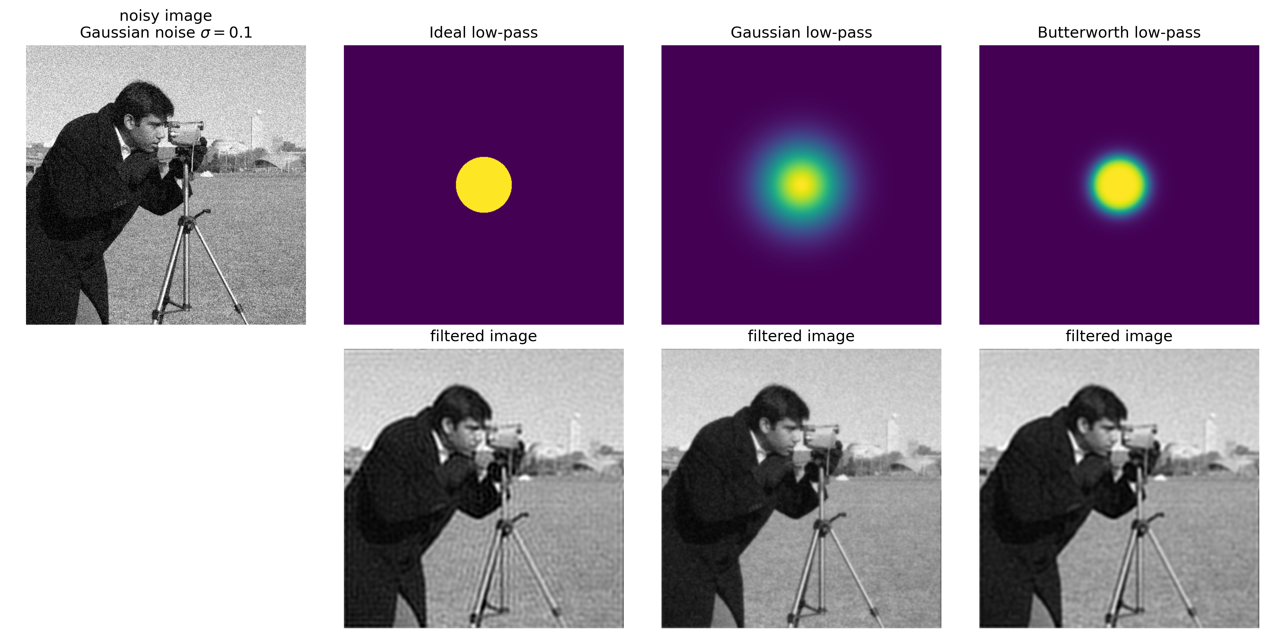
An alternative view on the Gaussian filter is to consider it as weighting in the Fourier domain:

Convolution in the spatial domain is equivalent to multiplication in the Fourier domain.
This enables to efficiently filter large images with a wide variety of filters.

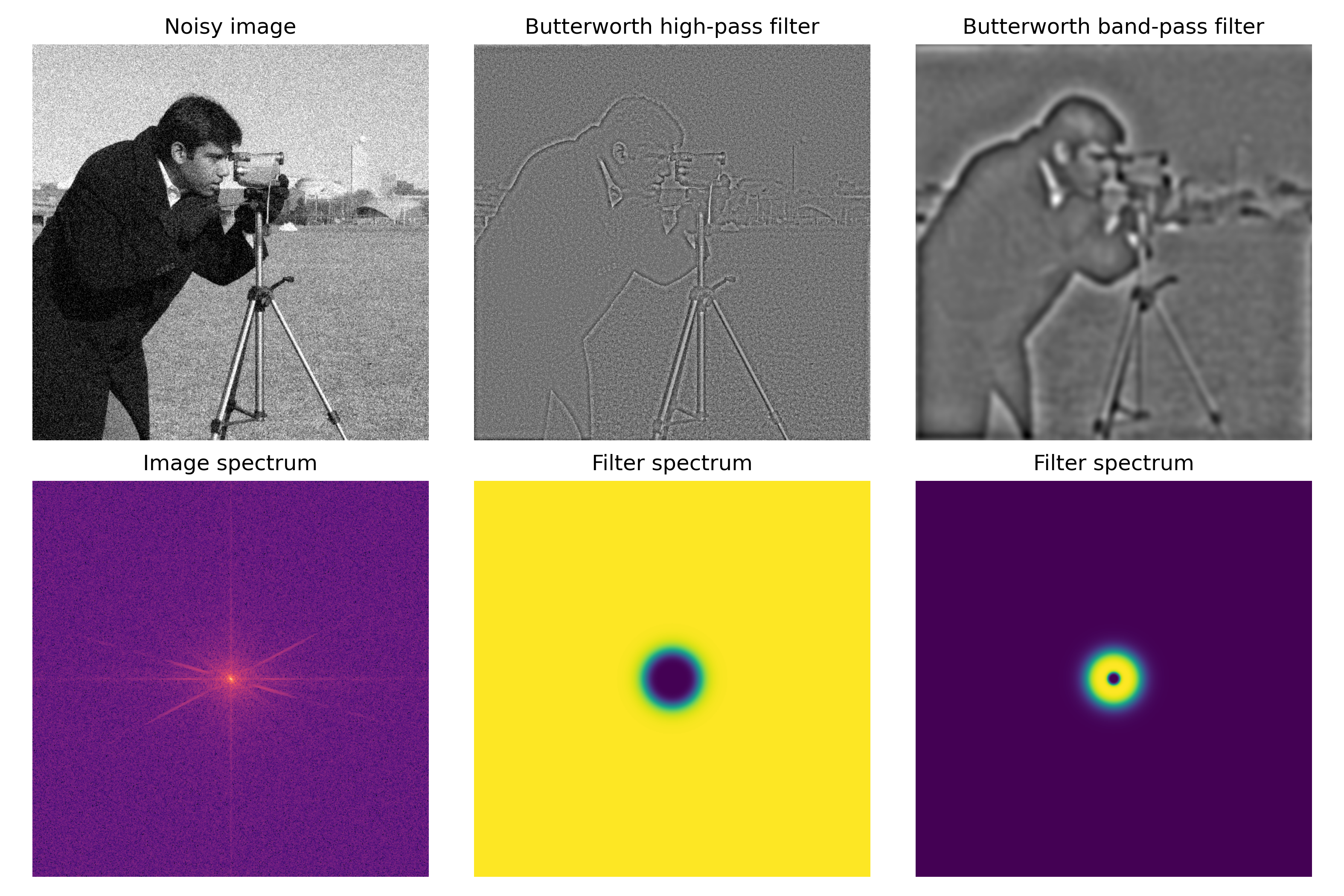
Fourier domain provides an intuitive representation for constructing different filter types:

Transform-domain methods¶

So far, we have treated image in the natural pixel-basis and the Fourier basis.
We have also seen both linear and non-linear filters.
These ideas can be extended to transform-domain filters.

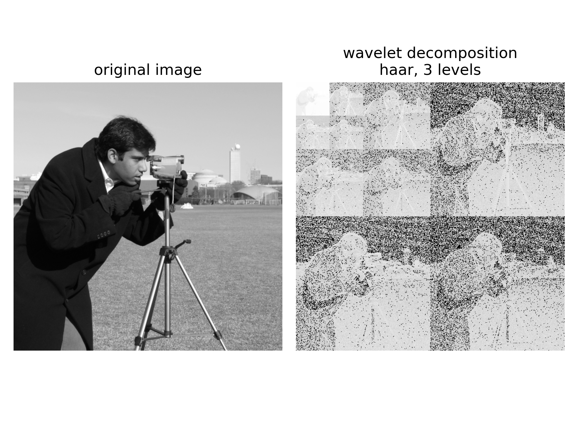
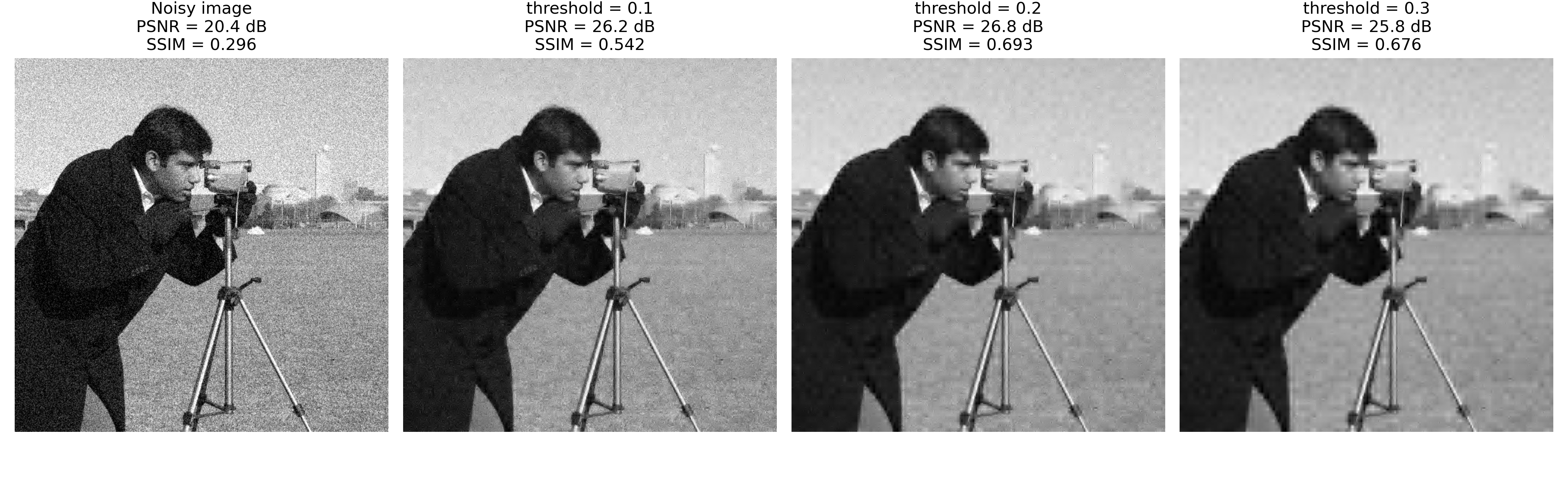
Wavelet transform

Decompose the image per scale, in a way that combined spatial location and frequency content.
Thresholding the image to keep only the coefficients with highest energy compresses the image (and hopefully reduces noise).
Can be implemented efficiently.

Singular value decomposition

The wavelet decomposition uses a fixed basis to decompose the image.
We can also make the basis dependent on the image.
Viewing the image as matrix, we can decompose it as: $$F = \sum_{i} \sigma_i u_iv_i^\top$$
The SVD algorithm is very efficient and widely used in many applications.

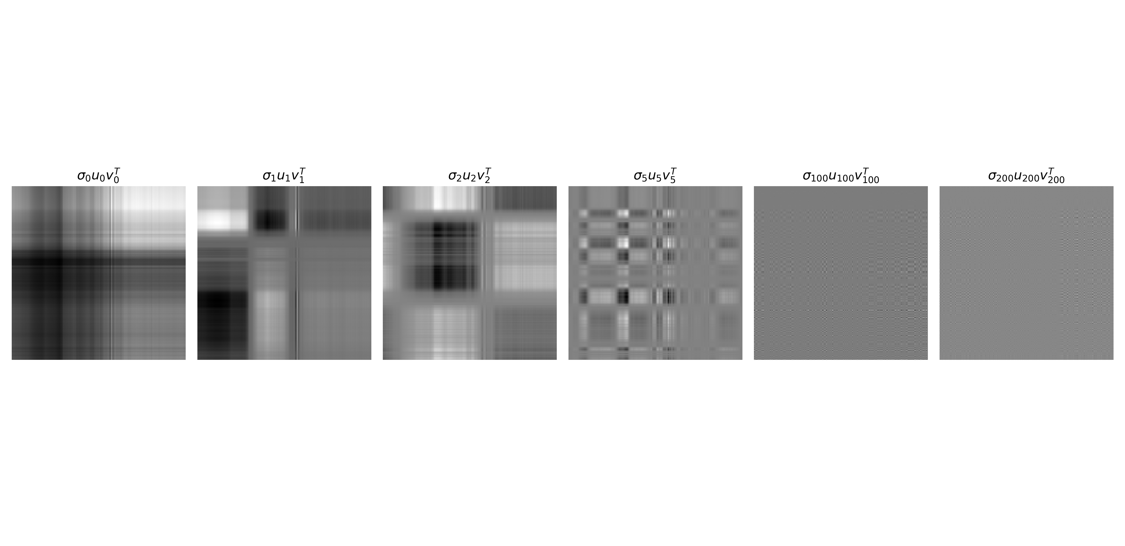
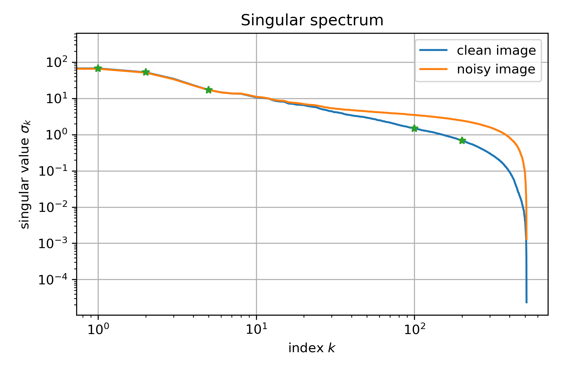
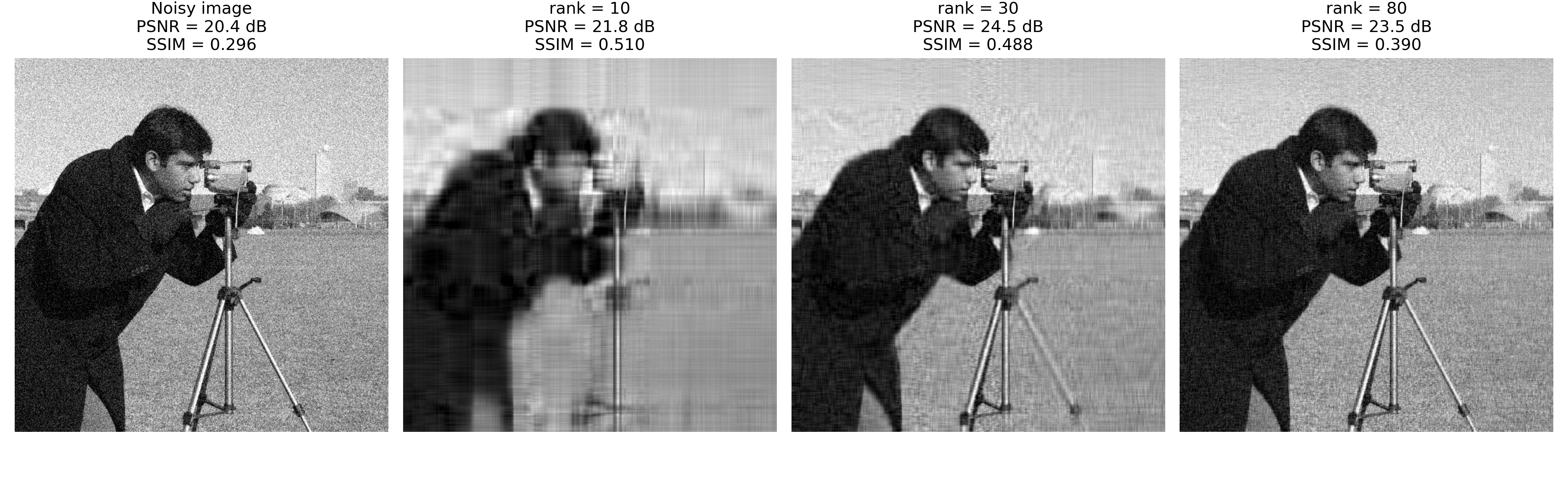
Usually, the singular values for the clean image decay rapidly, while the noise has a flatter spectrum (less structure):

This allows us to denoise the image by keeping only the components with the largest singular values:

Variational denoising¶

Model denoising as a balance between fitting the measured data and enforcing prior structure: $$\min_{F} \mathcal{D}(F,F^\delta) + \lambda \mathcal{R}(F),$$
Here $\mathcal{D}$ is the data-fidelity term, determined by the noise model, and $\mathcal{R}$ is the regularizer, encoding prior assumptions on plausible images.
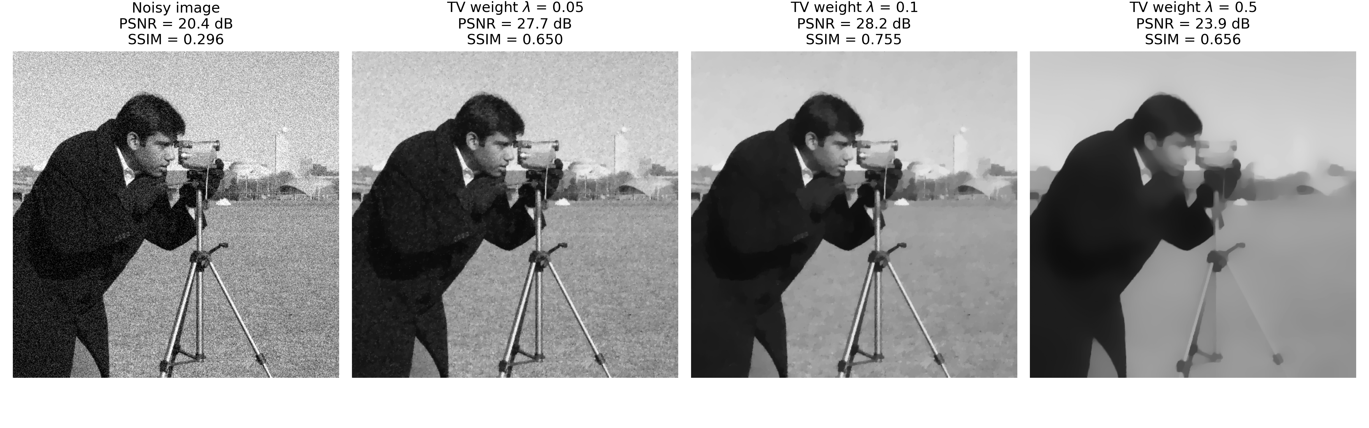
Increasing $\lambda$ usually gives more stability and lower variance, but also more bias.

Solving them may not be trivial (contact your local mathematician 🙂).
Most algorithms solve iteratively, and contain algorithmic parameters that need to be chosen carefully.
Care needs to be taken when picking the regularization weight $\lambda$.

We can adapt this formulation based on the noise and object model. Common examples:

Gaussian noise: $\mathcal{D}(\mathbf{f},\mathbf{f}^\delta) = \|\mathbf{f} - \mathbf{f} ^\delta\|_2^2$
Poisson noise: $\mathcal{D}(\mathbf{f},\mathbf{f}^\delta) = \sum_i f_i - f_i^\delta \log(f_i)$
Object sparsity (few non-zero pixels): $\mathcal{R}(\mathbf{f}) = \|\mathbf{f}\|_1$
Object smoothness: $\mathcal{R}(\mathbf{f}) = \|\nabla \mathbf{f}\|_2^2$

Many of the denoising approaches mentioned earlier can be modelled in this way:

Linear filters: $$\min_\mathbf{f} \|\mathbf{f} - \mathbf{f}^\delta\|_2^2 + \lambda \|L\mathbf{f}\|_2^2$$
Wavelet tresholding: $$\min_\mathbf{f} \|\mathbf{f} - \mathbf{f}^\delta\|_2^2 + \lambda \|W\mathbf{f}\|_1$$
SVD tresholding: $$\min_F \|F - F^\delta\|_\text{frobenius}^2 + \lambda \|F\|_*$$

A well-known example is Total Variation (TV) denoising with:

$$\mathcal{D}(\mathbf{f},\mathbf{f}^\delta) = \|\mathbf{f} - \mathbf{f} ^\delta\|_2^2, \quad \mathcal{R}(\mathbf{f}) = \|\nabla \mathbf{f}\|_1.$$

It promotes sparse edges in the image (i.e. piece-wise constant images).
Robust algorithms exist, but are relatively slow compared to explicit filters.
Care needs to be taken with algorithmic parameters (tolerance, number of iterations).

Beyond...¶

Patches: Apply any of the methods to local patches of the image.
Dictionary learning: Learn a representation based on a training data set.
Deep learning: Can be seen a generalisation that learns a representation and how to threshold it.

Wrap-up¶

We can generally classify methods as linear and non-linear, local and global.
Many of the methods can be formulated as an optimization problem.
Whichever method you use, it strikes a balance between bias and variance.
Many well-understood classical methods for denoising exist -> try those first!
If you have training data, a next step could be to fine-tune a classical method to it (filter choice, parameter tuning, freeform learned filter).